Digital Media - Part 01 - Audio
Series Introduction
If you work with audio or video, even if only tangentially, it can be helpful to have some context around how this media is recorded, represented, and stored. The purpose of this series is to provide some of this context. It is not intended to be exhaustive, rather to provide enough background in one place while highlighting how the concepts relate to each other to allow you to research the different areas further.
- Part 1 - Audio (You Are Here!)
- Part 2 coming soon…
- Part 3 coming soon…
Sound
When an instrument produces sound, its vibration creates changes in air pressure that propagate out through the air. The more of these changes in pressure within a given time span, the higher the frequency. The larger the magnitude of these pressure changes, the louder we perceive it as being.
Analog vs. Digital
Imagine a band is playing a song in front of you. Their instruments all cause different changes in pressure, and these pressure changes propagate through the air and into your ears. The music you are hearing is analog; it is continuous, meaning that at any point in time, there is a particular amount of pressure that your ears are experiencing. If you want to know the exact amplitude of sound for all times during second 30 and second 31 of the song, you would need an infinite number of amplitudes measurements. When trying to make a digital representation of the sound we experience, we can’t have an infinite number of amplitudes. That would take an infinite amount of storage to store, an infinite amount of processing power to process, etc.
To make a digital representation of audio, instead of taking all possible measurements, we take a sample of them.
Sample Rate
Instead of trying to record an infinite number of amplitudes of the performance over time, we can instead sample the signal many times per second. This means that we take many measurements of the amplitude of the sound at specific times. If we later draw a line between the amplitudes measured, we can approximate the original analog signal.
How frequently do we need to sample the signal to make a good digital approximation of it? It depends on the maximum frequency you want to be able to represent in a digital recording. Some people smarter than myself figured out that you need to sample a signal at double the maximum frequency you want to represent. It is generally stated that humans are able to hear sound between 20Hz and 20,000Hz. Therefor, to record the maximum frequency that humans can hear, you to sample the signal 40,000 times every second. By far the most common sampling rate for music is 44.1kHz, or once every 2.268 microseconds. This can theoretically represent a maximum frequency of 22,500Hz.
A sampling rate you will typically see used for movies is 48kHz, which can represent a maximum frequency of 24,000Hz. This is just the value that is used as a standard, and it being higher than that typically used for music does not mean it provides a better listening experience.
Each sample takes a particular amount of data to represent. This means that as the sampling rate increases, so does the resulting file.
20Khz is really the absolute upper bound of human hearing, and your ability to hear frequencies anywhere near this tend to diminish as you age. As someone who listens to a song or watches a movie, there is no reason to seek out audio with a higher sampling rate than 44.1kHz or 48kHz unless the only format available is higher. You won’t be able to hear the additional frequencies that a higher sampling rate can capture. Some people will use the bigger number to get you to pay more for the audio, but this provides no benefit to you. There are some scenarios in the audio mixing process that can benefit from a higher sampling rate, but this does not apply if you are just listening to the audio. For further convincing, see this excellent post by Monty Montgomery, founder of the Xiph.Org Foundation.
Bit Depth
When taking these samples of signal amplitude to make a digital representation of the audio, we run into another case that would require an infinite amount of storage and processing power to process. Say we measure the amplitude of audio on a scale from 0 to 1. There is an infinite amount of different numbers between these two values. Instead, we can say something like “a sample can be at an amplitude between 0 and 1 rounded to the nearest 0.1. This means that there are only 11 possible values (0.0, 0.1, 0.2, 0.3, 0.4, 0.5, 0.6, 0.7, 0.8, 0.9. 1.0) for an amplitude measurement.
Because of how computers represent numbers, we would need 4 bits of data to represent the above sample that can be in one of the 11 possible states. You can imagine that only being able to represent 11 possible amplitudes of sound would not allow us to be very accurate in capturing the true amplitude of sound with any of our samples. That’s why the most common format allocates 16 bits to each sample. This allows for 65536 possible values, which allows the sample to be accurate enough to the original amplitude that you will not hear the difference.
Each sample takes this number of bit to represent. This means that as the bit depth increases, so does the resulting file.
Much like sampling rate, people will try to charge you more money for audio with a higher bit depth higher than 16 bits (commonly 24 bits). Again, you will not be able to perceive any difference between the two.
Volume
To describe the volume of sound, we use different forms of the decibel (dB) unit. This is a logarithmic unit that is used due to the logarithmic nature of sound.
Decibels are a relative unit, meaning they require a reference point to compare with. This reference point can vary depending on the use case. You can’t say that a sound is x dB in isolation; it needs to be x dB louder or quieter than a reference point.
There are many uses of the decibel, but most of them are not relevant to audio. The most relevant of them for this post are:
- dB SPL
- dBA
- dBFS
Confusingly, in the context of audio, the specific name of the unit in use is not always mentioned, and instead a generic “dB” is used. It’s likely that it is referring to one of the three above units, but determining which one is in use can depend on the context it’s used in.
dB SPL
dB SPL (sound pressure level) is the standard way to refer to the amplitude of a sound. As mentioned, decibels require a reference point to compare the measured sound’s amplitude to. In the case of dB SPL, this reference point is 20 μPa which is considered to be the quietest sound that the average human can hear. Therefor, it can generally be assumed that positive dB SPL values can be heard by most humans, while negative dB SPL values can not be heard by most humans.
As decibels are a logarithmic unit, a doubling of the value does not always mean a doubling in volume. Instead, in the context of audio, +6 dB represents a doubling in volume, and -6 dB represents a halving of volume.
dBA
dBA (A-weighted) refers to a variant of dB SPL that is weighted to account for nonlinearity in how humans perceive loudness. Due to the physical properties of the human ear, some frequencies are perceived as quieter than others even at the same dB SPL level. A-Weighting is used to weight the volume of a sound in dB SPL to better represents the volume as perceived by a human.
This unit is very common in the context of safe and unsafe volumes as they relate to humans. Generally, humans perceive low frequency and high frequency sounds as quieter than frequencies closer to the mid-range of their perceptible range at the same dB SPL level.
dBFS
dBFS (Full Scale) is a unit commonly used in digital audio production. The loudest sound that can be represented in in the given digital form is referred to as 0 dBFS. All other amplitudes are referred to with negative dBFS values relative to this 0dBFS reference point.
As described in the Bit Depth section, we have a finite set of values that we can use to represent the amplitude of the signal at any point in time. For 16 bit audio, this is 65536 values. The highest value we have access to is 65535 to, so it would be the 0 dBFS reference point when viewed in an audio editor. 0 is the lowest value we have access to. This represents a volume -96 dBFS lower than 0dBFS. Therefor, 16 bit audio has a maximum range of 96 dB.
In a 24 bit audio file, we have 16,777,216 values to represent the amplitude of a signal. This gives us a range of 144 dB. Digital audio production software commonly use 32 bit floating point values which provide a range of 1528 decibels. This massive amount of range has utility in digital audio production as it allows more manipulation of the signal with less degradation. As someone listening to the finished audio, however, you do not benefit from this increased range as most of this range is too quiet to be perceived at normal listening levels.
Dynamic Range
Dynamic range is the “distance” between the quietest sound in a recording and the loudest sound. If you have a recording of both whispers and shouts, you generally will want them to play back true to life. The whispers should be very quiet, and the shouts should be very loud. If they were both the same volume, you could still hear both, but you would lose this distance between their volumes.
Having a high dynamic range (meaning a large distance between the quietest and the loudest sound) in music is generally a good thing, as you have more “room” to represent different volume levels. This will generally be one of the goals that the person mixing a track is aiming for.
Sometimes, too much dynamic range can be a bad thing. Have you ever watched a movie where the dialog is so quiet that you increase the volume, just for the music to kick in and and explosion to go off, rupturing your eardrums? This is a case where the distance between the quiet sounds (the dialog) and the loud sound (the music and explosion) are too far apart. I’ve read that the audio is mixed this way as to sound it’s best on high-end surround sound speaker setups where is supposedly sounds much better, but as someone without high-end speakers, it can be very annoying! If this happens to you, some TVs and stereos have compression filters that can reduce the amount of dynamic range which can somewhat resolve this issue.
Audio Channels
Audio files can contain one or more channels of audio data, which are each separate streams of audio data.
The most simple form of an audio recording is mono, meaning that it uses a single channel of audio. An individual microphone will generally produce a mono audio stream. When listening to a mono audio file with headphones, the same audio track is played from each speaker at the same time.
The vast majority of music today is available with stereo channels, meaning that there are two separate audio streams contained within the audio file. One stream is designated as the left channel, while the other stream is designated as the right channel. When listening to a stereo audio file with headphones, the left channel is played from the left speaker and the right channel is played from the right speaker. This allows for a few different techniques that can improve the experience of listening to the audio:
- Certain sounds can be played to one ear or the other. An example of this can be heard in the intro of Ain’t no Rest for the Wicked by Cage the Elephant
- Through using two microphones while recording, it can sound like you are in the environment where the audio was recorded. Instruments can sound like they originate from different locations. This effect can be particularly dramatic through the use of Binaural Recording. A human head shaped model with microphones located in the ears of the model can produce a recording that allows the listener to have an accurate understanding of where sounds are coming from in relation to their head. A classic example of this is the Virtual Barber Shop.
The use of more than two audio channels is referred to as surround sound. This is most commonly used with the audio for movies, however there does exist music that also uses surround channels. Surround speaker configurations involve positioning multiple speakers in certain locations around the listening location. You may have experienced a surround speaker configuration at a movie theater. Sounds can play from different speakers so the listener(s) have a sense of their directionality. Additionally, particularly with bass-heavy sounds like an explosion, you can physically feel the pressure of the sound acting on your body in addition to hearing it.
There are many different speaker configurations that are used for surround sound. One common way of describing these configurations are through writing “x.y” or “x.y.z”, where x refers to the number of primary speakers, y refers to the number of subwoofer speakers, and z refers to the number of overhead speakers.
- 2.0 refers to normal stereo audio
- 2.1 refers to stereo audio with a dedicated subwoofer for low frequency sounds
- 5.1 refers to having a front left, front right, front center, surround left, surround right, and dedicated subwoofer speakers
- 5.1.2 refers to having a front left, front right, front center, surround left, surround right, dedicated subwoofer, left overhead, and right overhead speakers
Lossless Audio
The representation of audio I’ve covered in this post is Pulse Code Modulation (also known as PCM). There are other ways to represent digital audio, but they are more niche.
The most common format for uncompressed PCM audio is WAV. This format stores metadata about the audio like it’s sample rate and bit depth, as well as all the audio samples that make up the recording. This is just enough so that the audio can be played back correctly. One downside of this format is that the file size is very large due to the audio samples not being compressed at all.
Lossless compression formats are able to compress these samples without discarding any of the original data. This is comparable to a zip file. If you create a zip file containing some documents (through a process called encoding), you will end up with a file that is smaller than all the files contained within. When you unzip the file (also known as decoding), you get back your original, unmodified, fully intact documents. The trade-off of this is that the encoding and decoding process takes some processing to convert between format. Typically, using less space at the expense of some additional processing time is beneficial.
Consider streaming music on your phone; you might have a data plan that charges you more as you use more data. Your phone is just sitting there in your pocket not doing much processing most of the time. Through the compression of the audio sent to your device, you will use less of your data plan (which costs money) while your phone just needs to use a tiny amount of electricity (which is essentially free in this amount) to decode the compressed audio.
The de-facto standard for losslessly compressed audio is the FLAC format.
Lossy Audio
Human hearing is imperfect. We generally can’t hear anything above 20kHz, and that limit decreases as we age. We can’t distinguish between frequencies if they are very close to each other. These facts and more are used to determine what parts of the audio signal can be discarded such that the listener will not notice at all or very much. The benefit of discarding this information is in huge reductions in the size of audio files at the same perceived level of quality.
Unlike lossless compression like with zip files, it is impossible to return the contained data to its original state. If upon unzipping your documents, you were to find that some letters were swapped or removed entirely, you would be understandable upset. With audio however, because of the space savings and how the discarded data can be targeted to be primarily data that you will not notice anyways, this can be a good trade off in exchange for much smaller file size.
Lossy formats will typically have quality levels that can be selected from to specify your desired mix of file size and audio quality.
This loss of data can be a problem for preservation of the original recording. While you may not hear the difference, the data that is lost has value, and this can be important.
The most common lossy format for music is MP3. Through the advancement of lossy audio compression technology, we now have formats that can match or exceed the same level of quality while further reducing the file size. MP3 remains in use today simply due to people’s familiarity of it and the support of the format by existing hardware.
The current best format for lossy music if your hardware supports it is Opus.
Transcoding
The process of converting between different formats is known as transcoding. There is different software available to perform this transcoding depending on the source and output formats.
Because the original audio can’t be re-generated from a lossy audio file, there is the concept of a “good transcode” and “bad transcode”.
Good transcodes allow you to either convert between different lossless formats, or correctly generate a lossy audio file. Converting a lossy audio file to anything else is a bad transcode. Bad transcodes from lossy to lossy result in audio of poor quality with no additional benefit to file size. Bad transcodes from lossy to lossless misrepresent the audio as originating from a lossless source.
Good Transcodes
- lossless -> lossless
- lossless -> lossy
- lossless -> lossless -> lossy
Bad Transcodes
- lossy -> lossless
- lossy -> lossy
- lossless -> lossy -> lossless
Spectral Analysis
Generally, you are not listening to a single sine wave at a particular frequency at a particular volume. Instead, you listen to songs that have different instruments outputting sounds at many frequencies and volumes. From the perspective of a microphone, all we can record is the changes in sound amplitude over times. At first this seems like we are losing all frequency information and only recording volume information, but by simply measuring the amplitude of pressure over time, you are capturing the different frequencies of sound within your recording. You can see these different frequencies with a spectral analyzer. A spectral analyzer is a piece of hardware or software that performs a Discrete Fourier transform on the audio. This converts our samples of amplitude over time into a distribution of frequencies. This happens many times over small windows of time, resulting in an approximation of how the distribution of frequencies in the recording change over time.
This is difficult to visualize without an example.
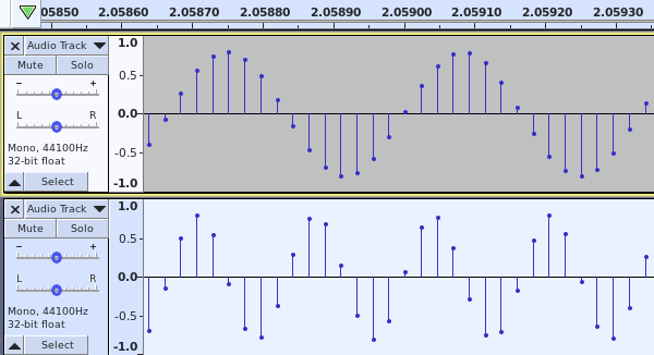
I’ve generated two tracks: a 3 kHz sine wave (top) and a 6kHz sine wave (bottom). You can see that the period of the 6 kHz sine wave is half that of the 3kHz sine wave.
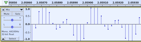
I then mixed the two tracks into a single track. The resulting waveform is a combination of to two source waveforms. It appears that we’ve lost the frequency of the two source signals, but it can be revealed again through spectral analysis.
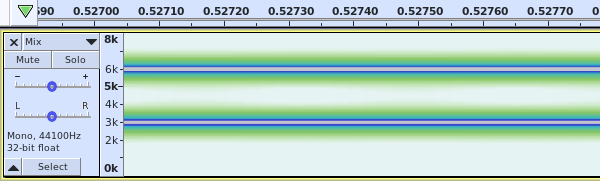
Here is a spectral analyzer showing the mixed single track. The Y-axis now represents frequency instead of amplitude, and the color now represents amplitude. You can see that there are peaks of sound at 3kHz and 6kHz. This shows that our original frequencies are all preserved even when mixed into a single track. Our ears do essentially the same process, allowing us to hear all the frequencies that went in to a recording even if it’s only played back on a single speaker.
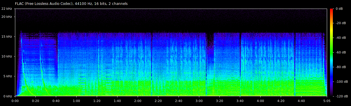
In a song, there are a lot more than two frequencies. This is how the song “I Ran” by A Flock of Seagulls looks in a spectrogram.
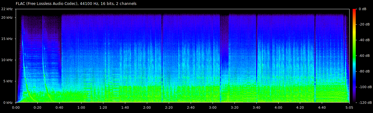
This spectrogram provides a key on the right side showing how the colors used relate to the amplitude of the signal at its different frequencies. You can visually see the pair of tones sweeping down in frequency near the beginning of the song. You can also see where the instruments stop for a moment at 2:11, 3:04, and 4:30.
Spectral analysis can also be used to identify bad transcodes like those described in the section on Transcoding. Here is the same song transcoded from a lossless FLAC file, to MP3 128 kbps, and then back to FLAC.
You can see that there is a shelf at around 16 kHz, above which there is no longer any sound. Removing high frequency sound that humans can’t hear very easily is one of the techniques used by lossy audio formats to save space. The lack of high frequency sound in a lossless format is an indicator that a bad transcode was performed.
Conclusion
At this point, you should have some understanding of the the most important parts of digital audio. If not, at least you have some terms to start researching more. It’s likely that not all of this will be relevant to you, and it’s also likely that I didn’t cover some topics that will actually be relevant to you, but I think this represents a good sample of what you may encounter.
I’m sure I’ve made a lot of errors in this post, so please let me know if you find any.
Thanks for reading!